How to read a phylogenetic tree
Tutorial | Phylogenetics
| Document: | ARTIC-Tutorial-Phylogenetics-Part1-v1.0.0 |
| Creation Date: | 2015-07-30 |
| Revision Date: | 2018-07-30 |
| Author: | Andrew Rambaut |
| Licence: | Creative Commons Attribution 4.0 International License |
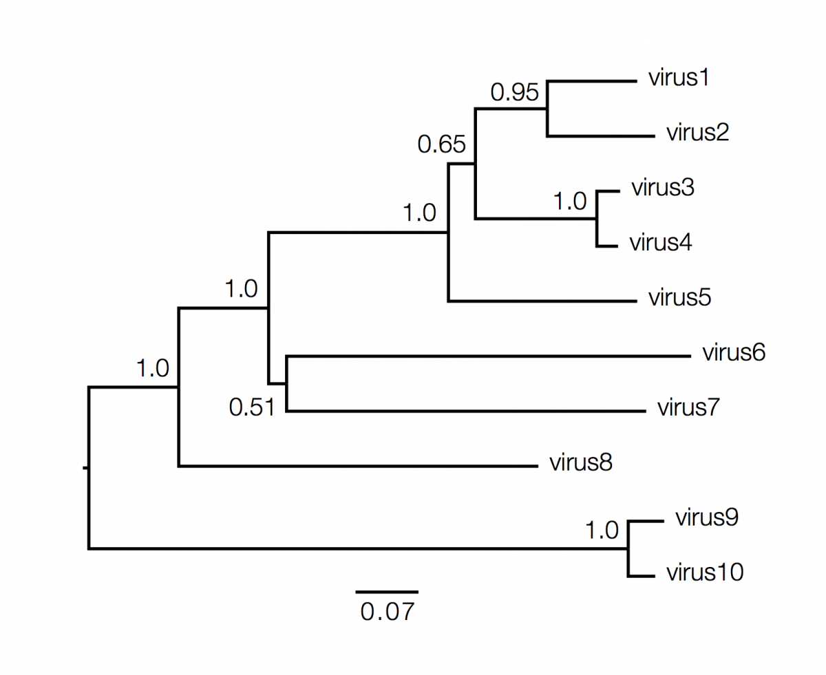
Phylogenetics trees contain a lot of information about the inferred evolutionary relationships between a set of viruses. Decoding that information is not always straightforward and requires some understanding of the elements of a phylogeny and what they represent. Here is an example (fictional) phylogeny as it may be presented in a journal article:
What information does the tree contain?
We can start with the dimensions of the figure. In this figure the horizonal dimension gives the amount of genetic change. The horizonal lines are branches and represent evolutionary lineages changing over time. The longer the branch in the horizonal dimension, the larger the amount of change. The bar at the bottom of the figure provides a scale for this. In this case the line segment with the number ‘0.07’ shows the length of branch that represents an amount genetic change of 0.07. The units of branch length are usually nucleotide substitutions per site – that is the number of changes or ‘substitutions’ divided by the length of the sequence (although they may be given as % change, i.e., the number of changes per 100 nucleotide sites). The vertical dimension in this figure has no meaning and is used simply to lay out the tree visually with the labels evenly spaced vertically. The vertical lines therefore simply tell you which horizontal line connects to which and how long they are is irrelevent.

Next, we will consider tree structure itself. This can be broken down into nodes (represented in the tree, above, as circles) and branches (the lines connecting them). There are two types of nodes; external nodes, also called ‘tips’ or ‘leaves’ (you can only take the tree metaphor so far and I prefer the term ‘tip’), and internal nodes. The tips are shown here with green circles and these represent the actual viruses sampled and sequenced. These are our data and we usually know information about these, beyond the actual sequence, such as when they were collected, what host they were in, where that host was found, clinical features of the disease.
The internal nodes are represented by blue circles and these represent putative ancestors for the sampled viruses. An ancestor in this context is an infected host at sometime in the past that in turn infected 2 or more new hosts producing chains of infections that lead to the sampled viruses. The branches then represent this chain of infections. This tree is rooted which suggests we know where the ultimate common ancestor of all the sampled viruses was (the red circle). Knowing this gives the tree an order of branching events in the horizonal dimension: Ancestor ‘A’ exists prior to ancestors ‘B’ and ‘C’ and time is approximately flowing from left to right. I say ‘approximately’ because in this tree the horizonal axis is measured as genetic change and to convert this into actual time we need to make some assumptions about the relationship between genetic change and time. These assumptions are referred to as the ‘molecular clock’ and I will discuss this in a later article.
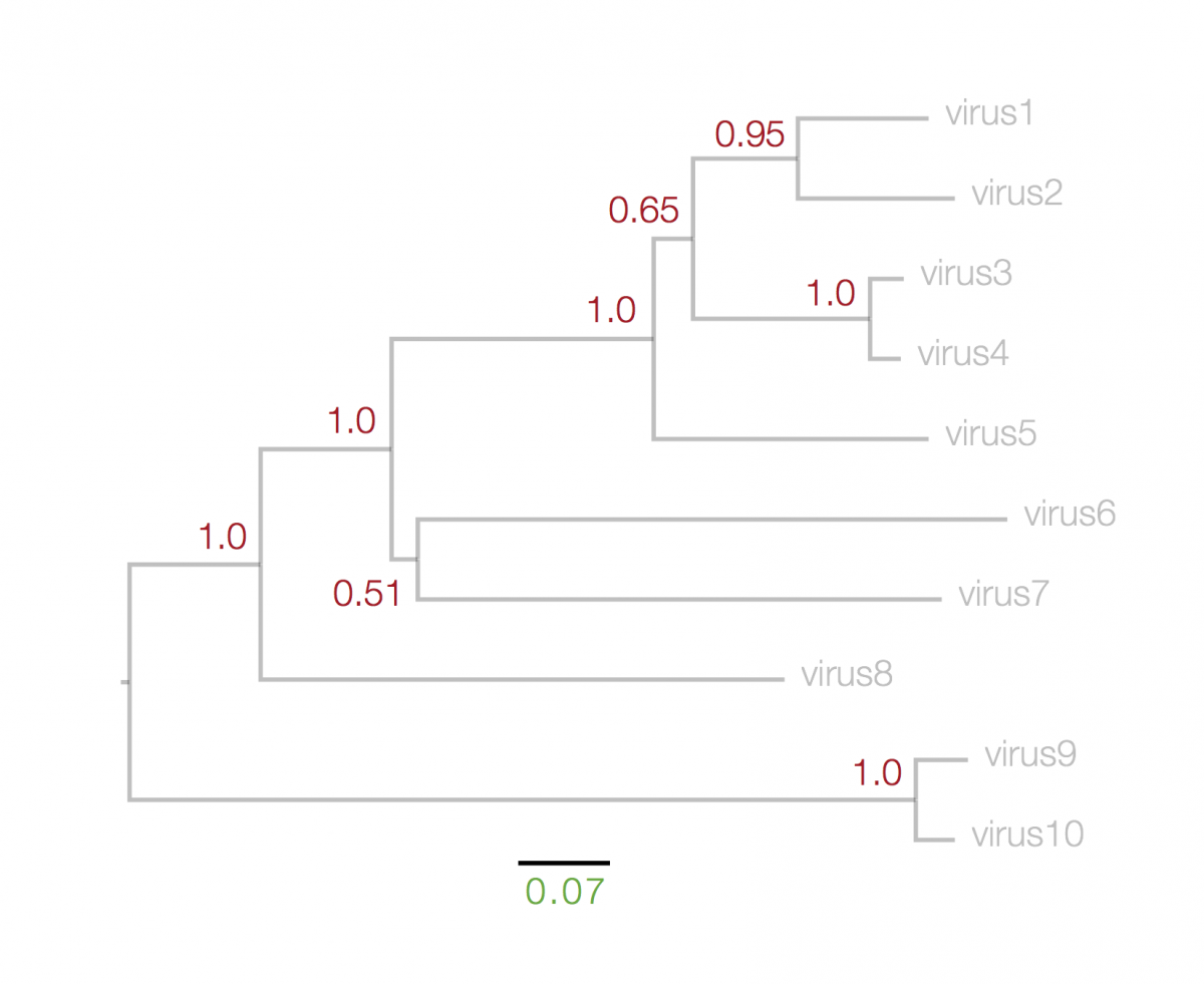
The numbers next to each node, in red, above, represent a measure of support for the node. These are generally numbers between 0 and 1 (but may be given as percentages) where 1 represents maximal support. These can be computed by a range of statistical approaches including ‘bootstrapping’ and ‘Bayesian posterior probabilities’. The details of what technique was used will be in the figure legend. A high value means that there is strong evidence that the sequences to the right of the node cluster together to the exclusion of any other.
Trees are sometimes drawn in other ways. Both these figures are representations of the same underlying tree as above:
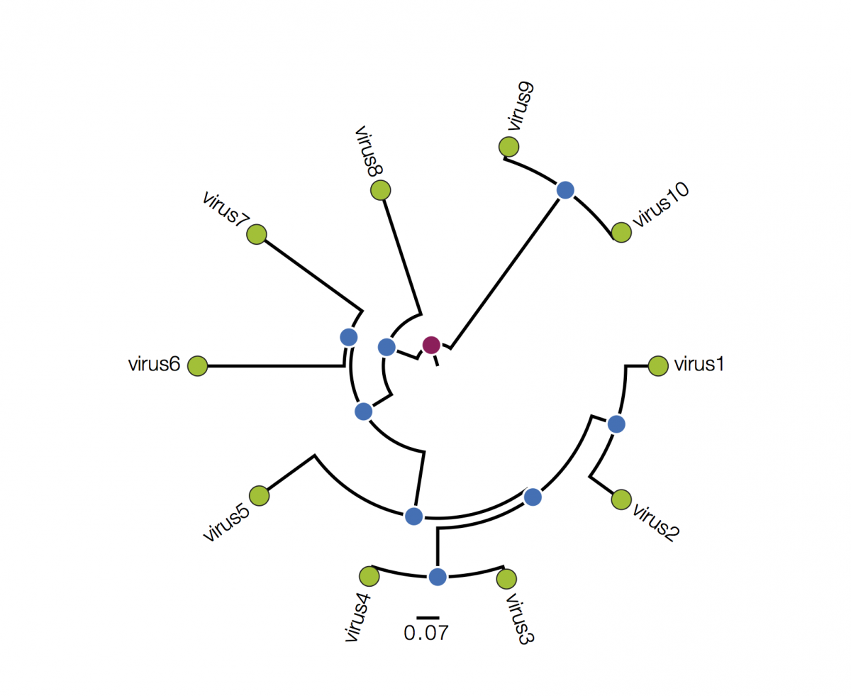
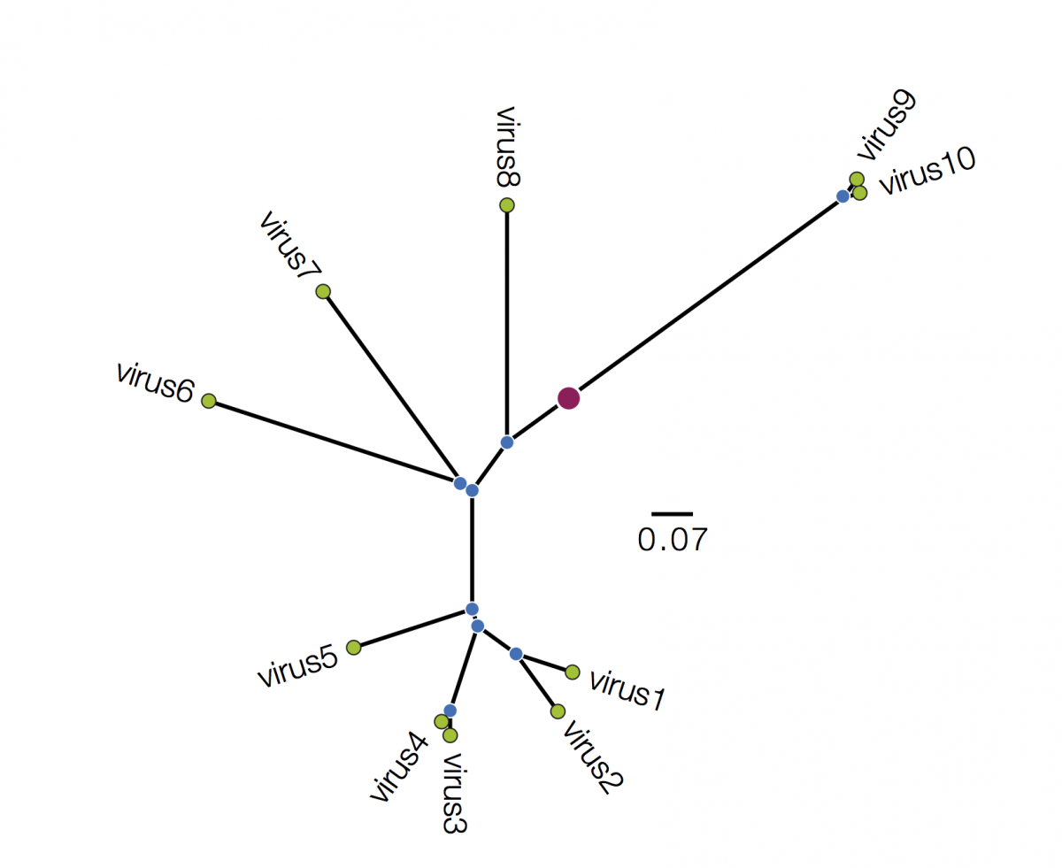
Tree A is in polar format (often called a circle tree). This is basically the same as the trees above but in polar coordinates. The vertical dimension is now the angle of the circle and the horizonal dimension is the distance from the centre point. These tree formats are often used to make a big visual impact in papers but generally have reduced readability - it is difficult to compare how far nodes are from the centre. They are best avoided. Tree B is a radial format tree. This is often used when the rooting of the tree is not known (although I have marked with a red circle the equivalent position of the root in trees above). This format tends to clump closely related sequences together making their precise relationships difficult to see. Generally best avoided too. I will not mention these formats again.
The root of the tree
I mentioned above that if we know the root of the tree then that provides information about the order of nodes in the tree. What do we do if we don’t know? How can we work out where the root is? Many methods of reconstructing phylogenies from gene sequences do not explicitly estimate the root of the tree. When the tree is generated it will often have an arbitrary root. For example, here is the tree, above, rooted in an arbitrary place:
This is exactly the same underlying tree as those above. I have marked the previous rooting position with a red circle. What is important to note is that it no longer holds that the left to right order of the internal nodes (the blue circles) can be interpreted as the order of common ancestors. Figures that are arbitrarily rooted should mention this in the legend but they often don’t. Click on the red circle and select Reroot on this node to switch the tree back to using this root.
How do we work out where the root is?
There are two ways of finding the root of a phylogenetic tree. The first is to include one or more sequences in the data set that are known to lie outside the diversity of the sequences of interest. These sequences are usually referred to as the ‘outgroup’. For example, in the trees above, the pair of tips labelled ‘virus9’ and ‘virus10’ could be the outgroup allowing us to root the tree at the red circle. How do we know the the outgroup is an outgroup? It is possible the outgroup has signficant genomic differences suggesting they are a different group of viruses. However, this might also mean the outgroup viruses are extremely divergent from the ones we are interested in. If the outgroups are too divergent from the sequences of interest then the root position will be unreliable. Alternatively it might be possible to assume that one or more sequences are the outgroup simply because they are the most divergent (virus9 and virus10, above, might be an example of this).
The second approach to rooting the tree is to use a method that implicitly assumes a time scale – a molecular clock model – as described below.
Reconstructing epidemiology
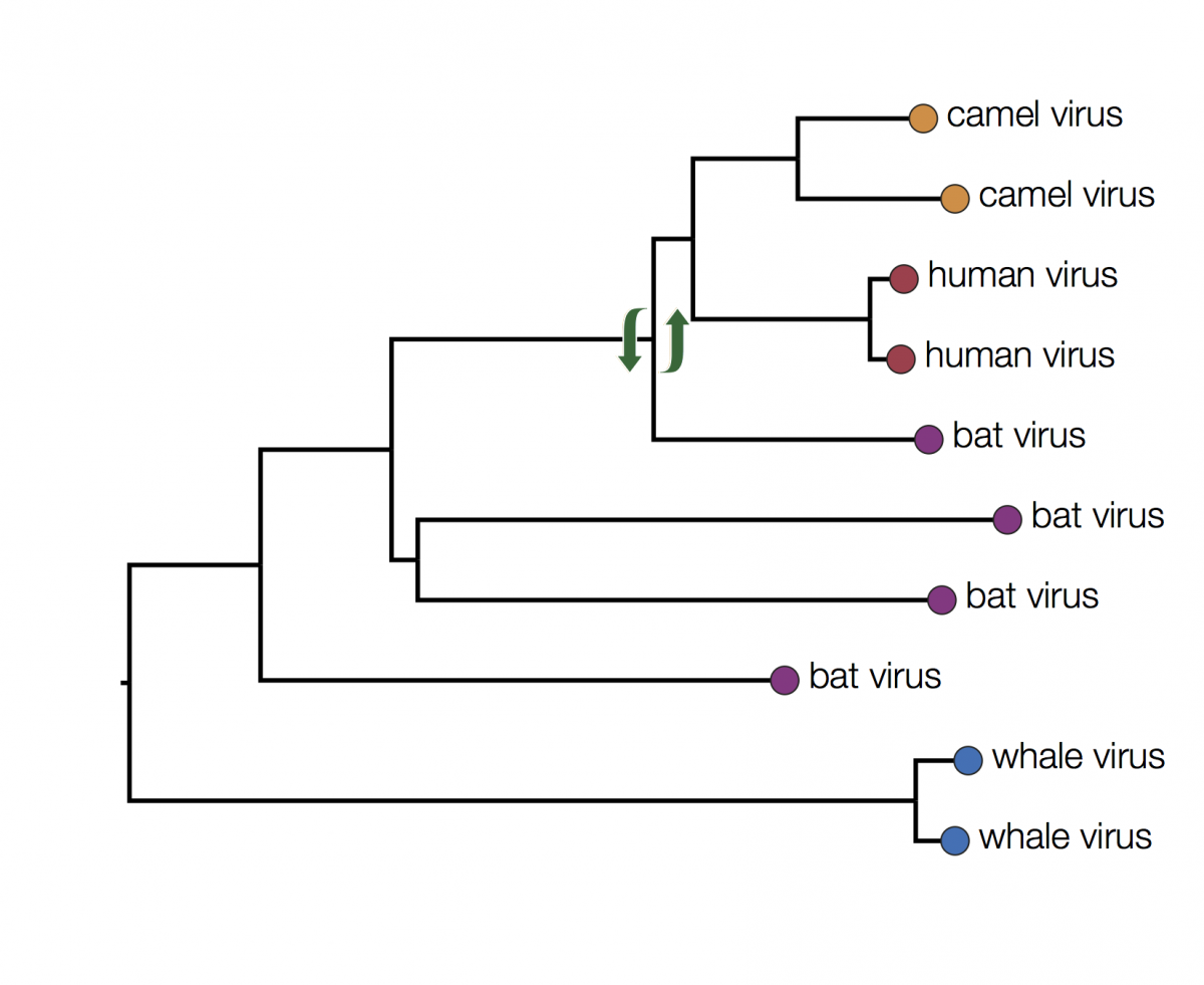
Here is the same tree as above but with the tips labeled by the type of host they were isolated from:

You can immediately see that there is some structure there with viruses grouping by host. For example the two viruses from humans have a closer common ancestor with each other than they do with any other virus. At first glance it may seem that human viruses are more closely related to bat viruses than camel viruses because they sit next to each other but remember that the vertical dimension is meaningless. In fact the viruses can be swapped round at any internal node and the tree is the same:
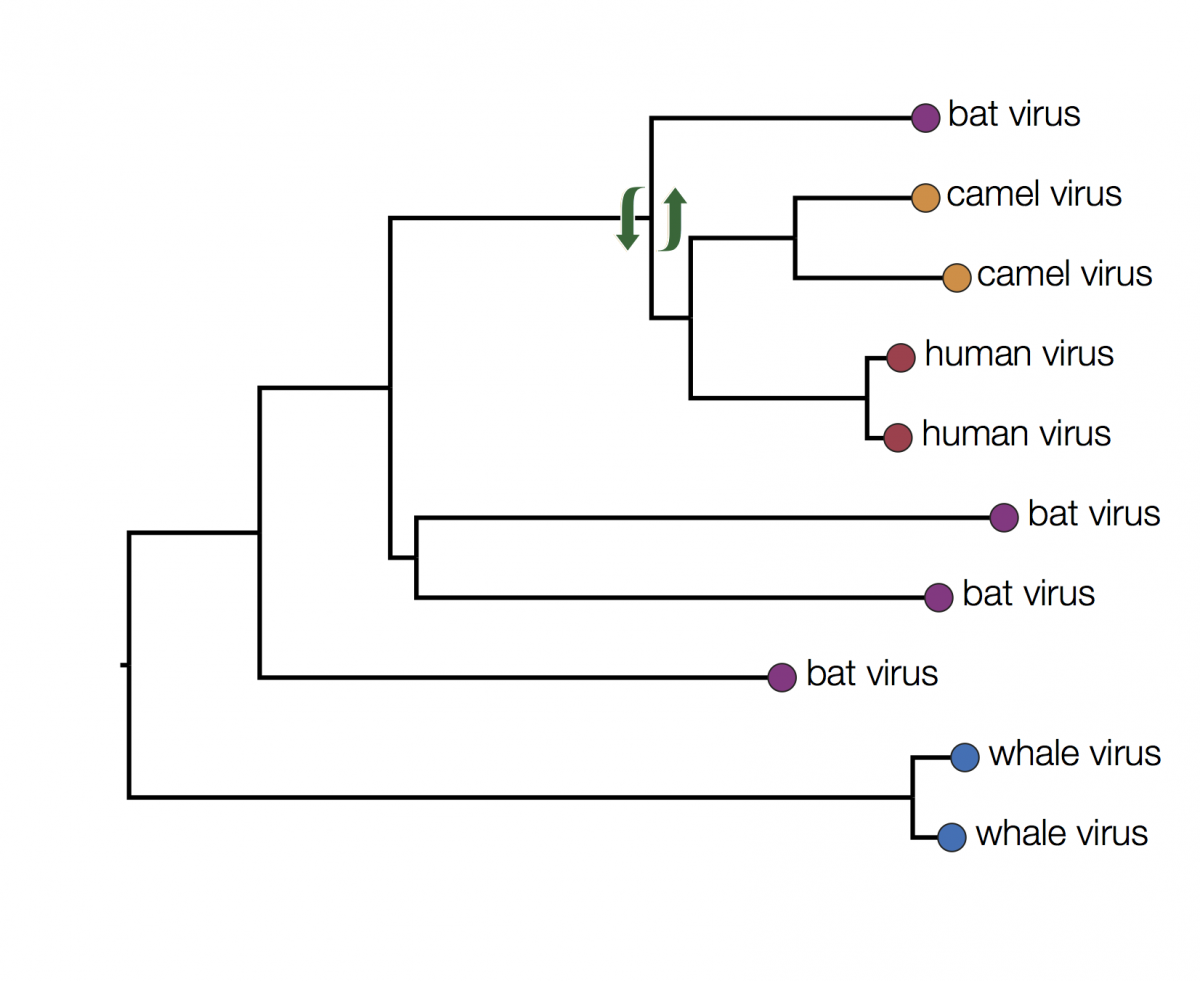
In fact the human and camel viruses are more closely related to each other and equally related to the bat viruses. This means we can’t say from this tree if camels are the source of the human viruses or vice-versa, or just as likely, bats are independently the source of both human and camel outbreaks. We can however suggest that bats were the ultimate source of both camel and human viruses because of the much greater diversity of bat viruses. Another way to look at this is that the common ancestors of the human and camel viruses lie within the diversity of all the bat viruses.
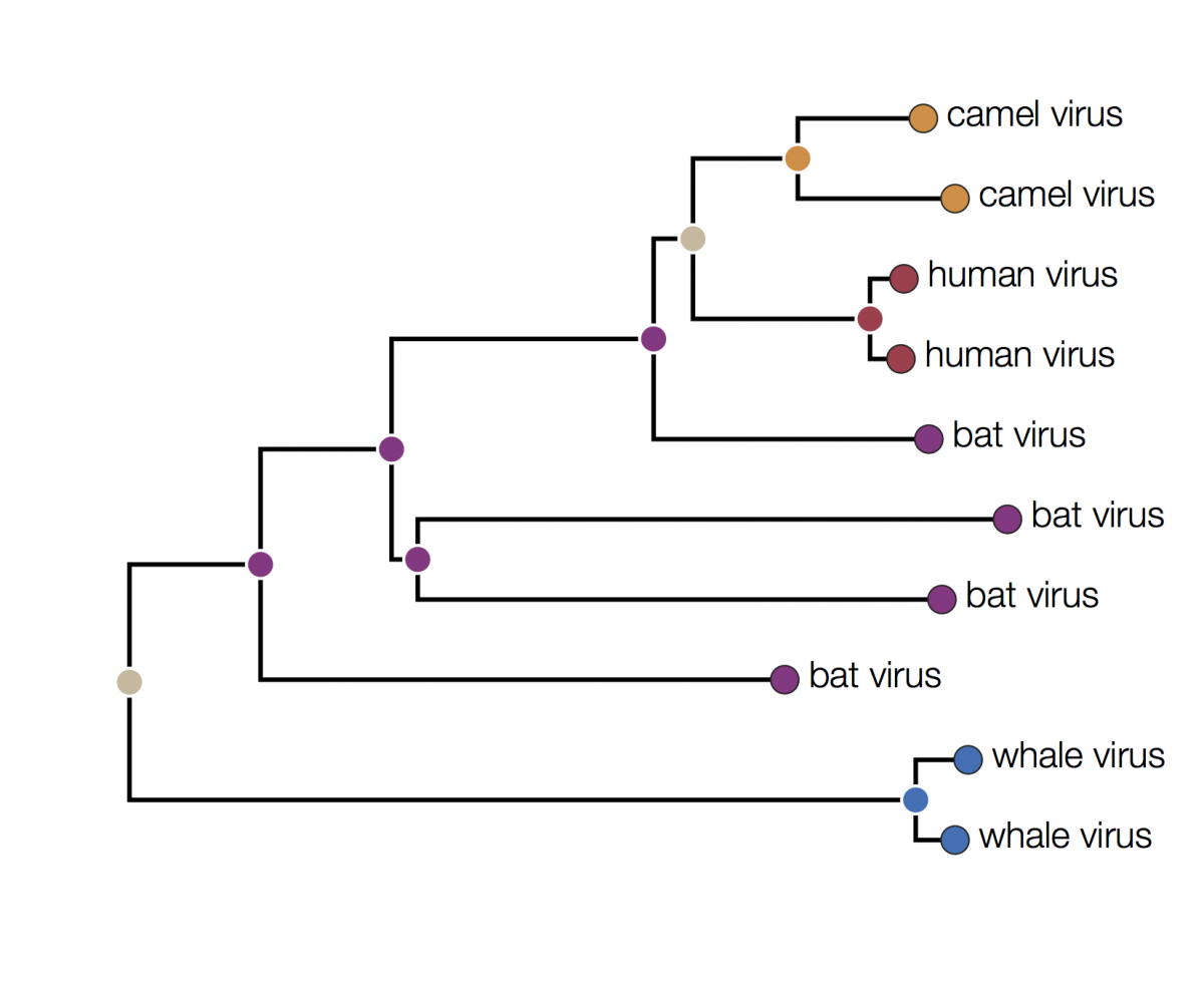
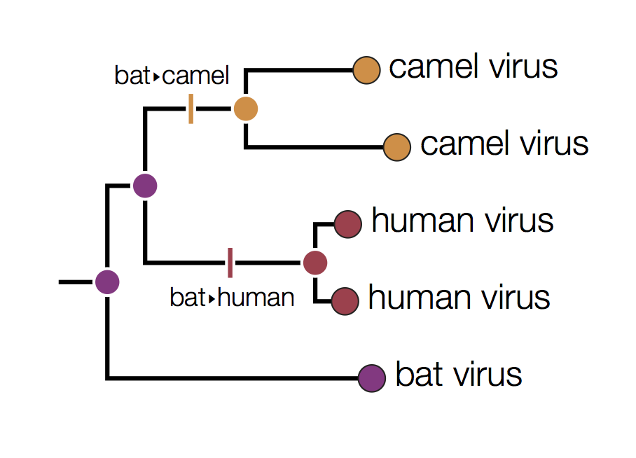
In this tree the internal nodes are labelled with the reconstructed host species based on the principle of parsimony. This is the reconstruction that requires the fewest jumps between host species. The grey nodes are those that cannot be unambiguously reconstructed. For example, the common ancestor of the human and camel viruses could equally well be in humans, bats or camels with all three possibilities only requiring 2 host jumps:
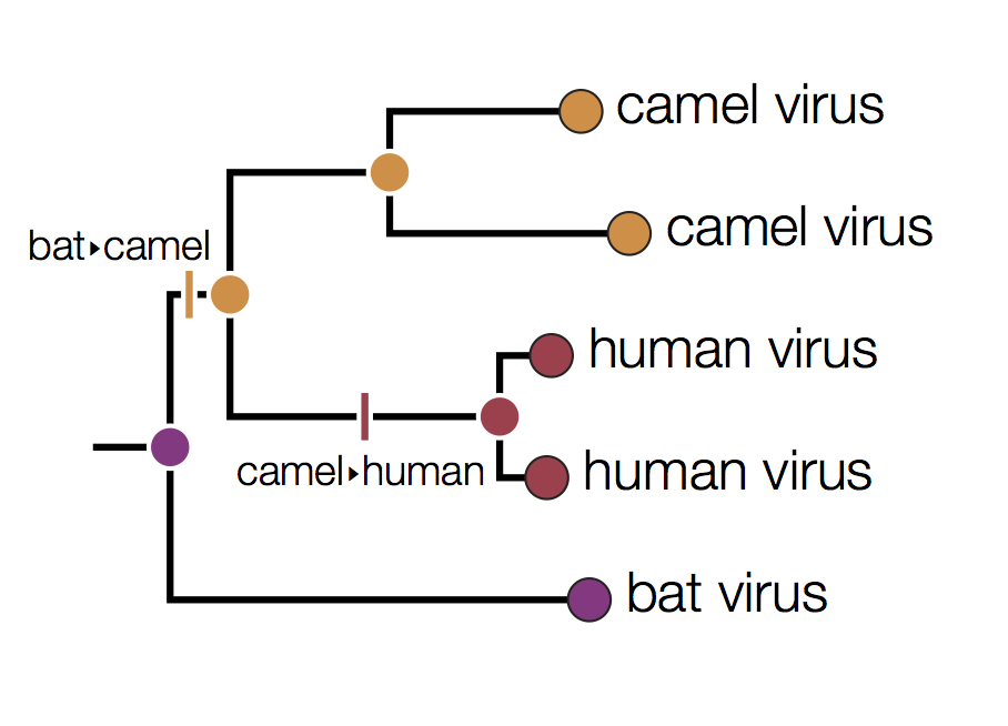
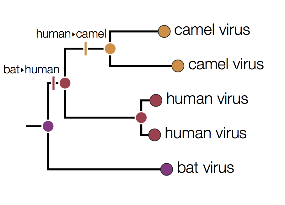
Distinguishing these three possibilities generally requires additional data perhaps with a denser sampling of viruses.