How to read a tree
Part 2: Estimating time scales using molecular clocks
| Document: | ARTIC-Tutorial-Phylogenetics-Part2-v1.0.0 |
| Creation Date: | 2021-07-11 |
| Last Updated: | 2025-08-27 |
| Author: | Andrew Rambaut |
| Licence: | Creative Commons Attribution 4.0 International License |
Phylogenetic trees usually have branch lengths in units of genetic change either as a count of the number of nucleotide differences or an estimate of the average number of changes per site in the genome. The latter estimates accommodate the fact that some of the genome may be missing in the sequence but the two are very similar when the number of mutations are small.
But in a transmission tree (which is ultimately what we are trying to infer for epidemiological inferences), the branch lengths are in units of time. The time units could be days, number of transmission events (assuming some expected duration between one transmission and the next - the ‘serial interval’).
Ultimately genetic changes occur when a virus is replicated in a cell so the rate of genetic change is dependent on the mutation rate (the rate at which mutations are introduced into the genome due to replication rate) and the number of cell-to-cell generations. The number of cell-to-cell generations between the virus that established an infection and the virus that is shed and establishes the next will be a function of time. So the number of genetic changes that a virus lineage acquires within a host will be a function of time, the mutation rate, and the probability of a virus with mutation going to high enough frequency to be transmitted. This is natural selection - most amino acid changes will cause a fitness loss and will have zero probability, a few might provide an advantage and go rapidly to high frequency, the rest will just end up being lucky.
Within the host, this rate will be fairly constant (it is reasonable to assume all the factors and processes in the paragraph above will remain the same) but outside the host the virus is not replicating so the rate is zero. This means that if the time spent in the environment is relatively small the amount of genetic change expected in a particular time in a transmission chain (a sequence of transmissions and infections) is simply the product of the within host rate of change and the total time (not the number of transmissions). This is likely to be the case with airborne respiratory viruses because transmission occurs by breathing out and breathing in viruses. For other viruses, transmission may occur through contact with surfaces and potentially this could involve significant time in the environment with no replication.
All of these processes have a considerable amount of variability in them. The number of mutations per genome replication is highly variable - RNA viruses generally have a mutation rate of about 1 error per genome. It may seem surprising that this is independent of genome length but generally viruses can’t tolerate too many mutations per replication or there will be a high likelihood of an unfit mutation occurring. On the other hand there is an advantage to the virus to replicate quickly and this is achieved through a polymerase that is error-prone. This trade-off means that viruses with short genomes can tolerate more errors per nucleotide than those with longer genomes.
As an aside, coronaviruses are one of the largest known RNA viruses but much of the extra space in the genome is made up of enzymes which assist in error-correction to allow them to have long genomes. But this may not be as circular as it seems because coronaviruses have a complex replication cycle so higher-fidelity RNA replication may be important in other ways.
Assuming an average of 1 error per genome, this will mean for a coronavirus (genome size of about 30,000 nucleotides) the mutation rate will be 0.000033 mutations/nucleotide/replication. Assuming a binomial distribution (a probability distribution that describes the number of times a particular outcome will occur given a fixed per ‘trial’ probability of the outcome happening and a certain number of trials) we find that per replication there is about a bit more than 1/3 probability that no mutations will occur, about the same that 1 mutation will occur and about 1/4 that more than one will occur (there is even a 2% chance that 4 or more mutations will occur).
Table 1 | Binomial distribution of mutation number for 30,000 nucleotides with a 3.3x10^-5 probability of mutation
| mutations | probability |
|---|---|
| 0 | 0.3679 |
| 1 | 0.3679 |
| 2 | 0.1839 |
| 3 | 0.0613 |
| 4 | 0.0153 |
| 5 | 0.0031 |
| >5 | 0.0006 |
Other sources of variability will be in the time between replication events, the probability of a mutation being transmitted, and potentially the length of time spent in the environment not replicating.
But ultimately this model of molecular evolution means that the number of genetic changes observed in a transmission chain is just a product of time and not the number of transmissions (if the time in the environment is small relative to time spent in the host). This is why we can estimate the time of the most recent common ancestor of an epidemic from a sample of viruses even if the rate of transmission and the number of infections is going up and down.
If we take the estimated rate of evolution as 0.001 changes per nucleotide site per year (this is not the ‘mutation rate’ but an observed rate of change estimated across the entire pandemic) we expect to get about 1 mutation in about 2 weeks (0.001 subst/site/year = 29 changes/genome/year = 0.56 changes/week). The other way of looking at it is that if we see 2 mutations on a branch this means this represents about 1 month of evolution. However, the large variability inherent in the process means that a wide range of other time periods are likely to give rise to 2 mutations.
This process (the accumulation of mutations at a fixed rate per time as a product of lots of individual, independent events) is often modelled with a Poisson process. Maximum likelihood and Bayesian software that allow for more sophisticated models of the evolutionary process use a continuous-time Markov chain (CTMC) but in its simplest form this is essentially similar.
The Poisson distribution gives you the expected number of events given an average rate of the events happening. The Poisson distribution for an expectation of 2.24 events (4 weeks of evolution at the rate above) is given in Table 2. You can see that although the most probable number of events is 2, 1 and 3 events have nearly as much probability and 0 and 4 have about 10% probability.
Table 2 | Poisson distribution for a rate of 0.001 subst/site/year = 29 changes/year = 2.24 changes/4 weeks
| changes | probability | cumulative probability |
|---|---|---|
| 0 | 0.1065 | 0.1065 |
| 1 | 0.2385 | 0.345 |
| 2 | 0.2671 | 0.6121 |
| 3 | 0.1994 | 0.8115 |
| 4 | 0.1117 | 0.9232 |
| 5 | 0.0500 | 0.9732 |
| 6 | 0.0187 | 0.9919 |
| > 6 | 0.0081 | 1.0 |
We can reverse this question and ask, if we see 2 mutations what amount of time could that represent? In 1 week we expect 0.56 changes and Table 3 gives the Poisson distribution with this mean. So we have > 50% chance of seeing no mutations, 32% of seeing exactly one, and still a 11% chance of seeing 2 or more.
Table 3 | Poisson distribution for a mean 0.56 changes (the number of changes expected in 1 week)
| changes | probability | cumulative probability |
|---|---|---|
| 0 | 0.5712 | 0.5712 |
| 1 | 0.3199 | 0.8911 |
| 2 | 0.0896 | 0.9807 |
| 3 | 0.0167 | 0.9974 |
| 4 | 0.0023 | 0.9997 |
| >4 | 0.0003 | 1.0 |
So one week of evolution still has a good chance of producing 2 mutations. In fact any amount of time between about 4 days and 13 weeks has a greater than 5% chance of producing exactly 2 nucleotide changes. Another way of looking at this is the 95% confidence intervals of the mean of a Poisson distribution for 2 observed events is between 3 and 90 days. Conversely a branch with no mutations (i.e., at a phylogenetic polytomy) can have a time span of between 0 and 46 days. A similar empirical observation can be made by looking at the span between sampling times of identical genomes in the SARS-CoV-2 pandemic (Figure 1).
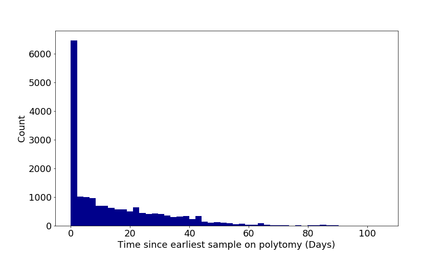
Figure 1 | Time spans between samples in sets of identical genomes relative to the earliest sampled genome of that set for the SARS-CoV-2 pandemic. Figure by Áine O’Toole, University of Edinburgh.
But unless we are sampling every single case it is very unlikely that we have sampled the genome at the beginning of the transmission chain so most likely any two genomes will share a most recent common ancestor MRCA at some point between them. So for two viruses sampled on the same day with 2 nucleotides difference between their genomes, their MRCA will have existed between 2 and 45 days prior to sampling. If they are not sampled on the same day then the MRCA will have existed proportionally closer to the earlier sample.
Notes:
A very nice online tool for calculating binomial and Poisson confidence intervals by John Pezzullo can be found here: https://statpages.info/confint.html